This document is a user-friendly manual on how to use the Treefit package, which is the first toolkit for quantitative trajectory inference using single-cell gene expression data. In this tutorial, we demonstrate how to generate and analyze two kinds of toy data with the aim to help get familiar with the practical workflow of Treefit. After learning some basics, we will use Treefit to perform more biologically interesting analysis in the next tutorial (vignette("working-with-seurat")).
1. Generating toy data
While the Treefit package has been developed to help biologists who wish to perform trajectory inference from single-cell gene expression data, Treefit can also be viewed as a toolkit to generate and analyze a point cloud in d-dimensional Euclidean space (i.e., simulated gene expression data).
Treefit provides some useful functions to generate artificial datasets. For example, as we will now demonstrate, the function treefit::generate_2d_n_arms_star_data() creates data that approximately fit a star tree with the number of arms or branches; the term star means a tree that looks like the star symbol “*”; for example, the alphabet letters Y and X can be viewed as star trees that have three and four arms, respectively.
The rows and columns of the generated data correspond to data points (i.e., n single cells) and their features (i.e., expression values of d different genes), respectively. The Treefit package can be used to analyze both raw count data and normalized expression data, but regarding the production of toy data, it is meant to be used to generate continuous data like normalized expression values.
Importantly, we can generate data with a desired level of noise by changing the value of the fatness parameter of this function. For example, if you set the fatness parameter to 0.0 then you will get precisely tree-like data without noise. By contrast, setting the fatness to 1.0 gives very noisy data that are no longer tree-like. In this tutorial, we deal with two types of toy data whose fatness values are 0.1 and 0.8, respectively. We note that Treefit can be used to generate and analyze high dimensional datasets but we focus on generating 2-dimensional data to make things as simple as possible in this introductory tutorial.
1.1. Tree-like toy data
Let us first generate 2-dimensional tree-like data that contain 500 data points and reasonably fit a star tree with three arms. We can create such data and draw a scatter plot of them (Figure 1) simply by executing the following two lines of code:
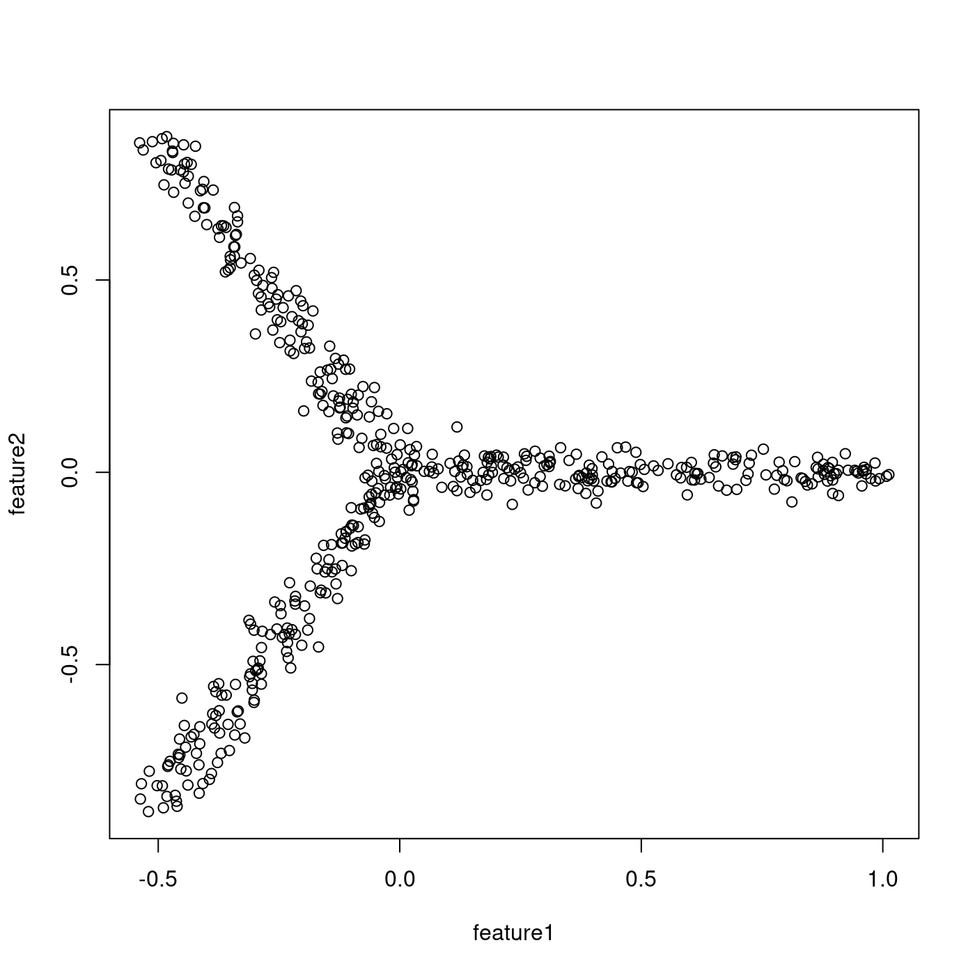
Figure 1. A scatter plot of tree-like toy data generated by Treefit
1.2. Less tree-like, noisy toy data
Similarly, we can generate noisy data that do not look so tree-like as the previous one. In this tutorial, we simply change the value of the fatness parameter from 0.1 to 0.8 in order to obtain non-tree-like data. The following two lines of code yields a scatter plot shown in Figure 2:
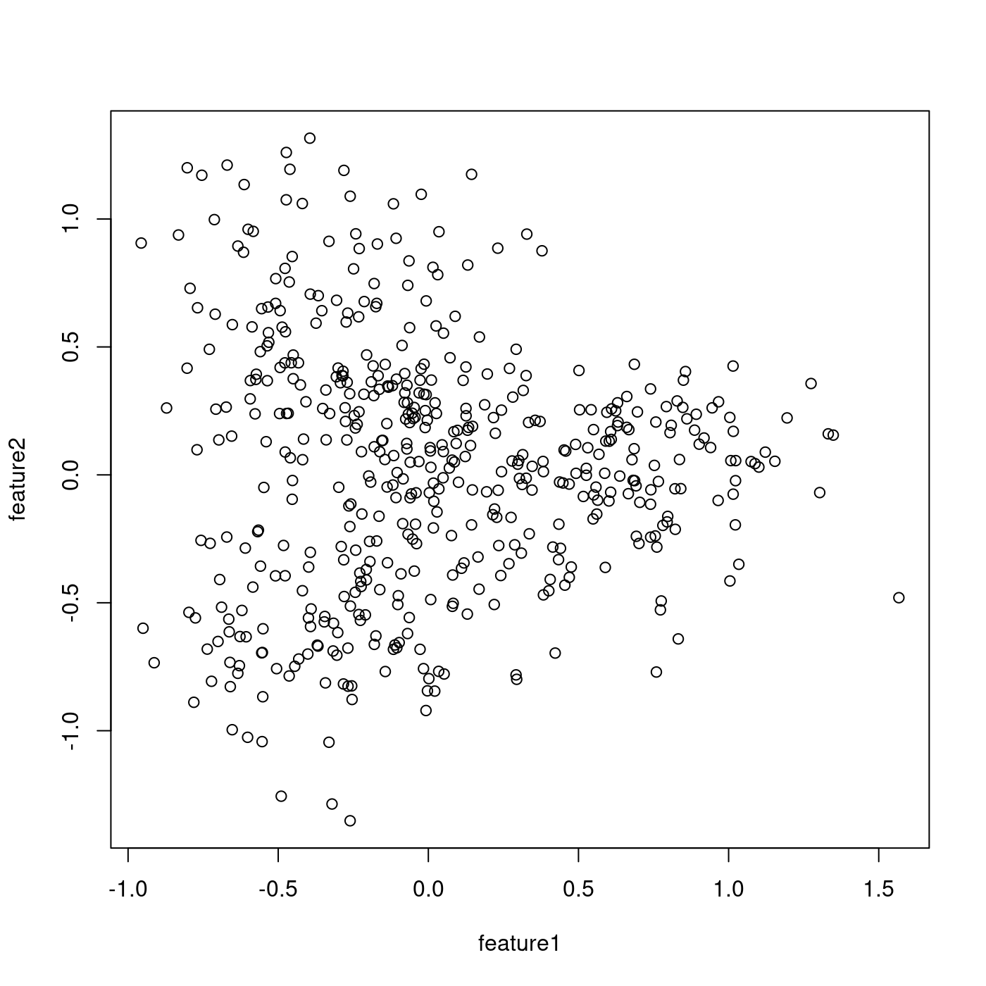
Figure 2. A scatter plot of noisy toy data generated by Treefit
2. Analyzing the data
Having generated two datasets whose tree-likeness are different, we can analyze each of them. The Treefit package allows us to estimate how well the data can be explained by tree models and to predict how many “principal paths” there are in the best-fit tree. As shown in Figure 1, the points in the first data clearly form a shape like the letter “Y” and so the data are considered to fit a star tree with three arms very well, whereas Figure 2 indicates that the second data are no longer very tree-like because of the high level of added noise. Our goal in this tutorial is to reproduce these conclusions by using Treefit.
2.1. Tree-like toy data
Let us estimate the goodness-of-fit between tree models and the first toy data. This can be done by using treefit::treefit() as follows. The name parameter is optional but we should specify it, if possible. Because it’s useful to identify the estimation.
fit.tree_like <- treefit::treefit(list(expression=star.tree_like),
                                  name="tree-like")
# Save the analytsis result to use other tutorials.
saveRDS(fit.tree_like, "fit.tree_like.rds")
fit.tree_like
## $name
## [1] "tree-like"
##
## $max_cca_distance
## p mean standard_deviation
## 1 1 0.15944808 0.080786824
## 2 2 0.06374979 0.010594737
## 3 3 0.05587648 0.008190445
## 4 4 0.04904369 0.007328796
## 5 5 0.04681459 0.006417239
## 6 6 0.04422028 0.006712903
## 7 7 0.04240203 0.006598741
## 8 8 0.03895063 0.007015447
## 9 9 0.03677757 0.005962633
## 10 10 0.03616917 0.005962774
## 11 11 0.03461220 0.006298050
## 12 12 0.03342942 0.006480975
## 13 13 0.03204465 0.006298932
## 14 14 0.03058407 0.006449666
## 15 15 0.02963478 0.006458244
## 16 16 0.02885938 0.006343777
## 17 17 0.02747453 0.006120983
## 18 18 0.02678371 0.005851636
## 19 19 0.02592523 0.006254678
## 20 20 0.02489788 0.006233318
##
## $rms_cca_distance
## p mean standard_deviation
## 1 1 0.031623874 0.031334581
## 2 2 0.006987244 0.002337299
## 3 3 0.010139801 0.002276433
## 4 4 0.022470646 0.008861128
## 5 5 0.022384100 0.006051647
## 6 6 0.029345338 0.009124936
## 7 7 0.038795822 0.015063872
## 8 8 0.061913017 0.018826334
## 9 9 0.056890818 0.016469581
## 10 10 0.073066508 0.020558640
## 11 11 0.095251498 0.033604789
## 12 12 0.105779269 0.029774827
## 13 13 0.108172778 0.023528394
## 14 14 0.144323355 0.019997741
## 15 15 0.136618158 0.026174061
## 16 16 0.162222369 0.025141011
## 17 17 0.171822259 0.034246384
## 18 18 0.168259433 0.030607172
## 19 19 0.179989614 0.028077026
## 20 20 0.190436948 0.027476754
##
## $n_principal_paths_candidates
## [1] 3 6 10 16 19
##
## attr(,"class")
## [1] "treefit"treefit::treefit() returns a treefit object that summarizes the analysis of Treefit. We will explain how to interpret the results in the next section. For now, we may focus on learning how to use Treefit.
As we will see later, it is helpful to visualize the results using plot(). By executing plot(fit.tree_like), we can obtain the following two user-friendly visual plots, which makes it easier to interpret the results of the Treefit analysis.
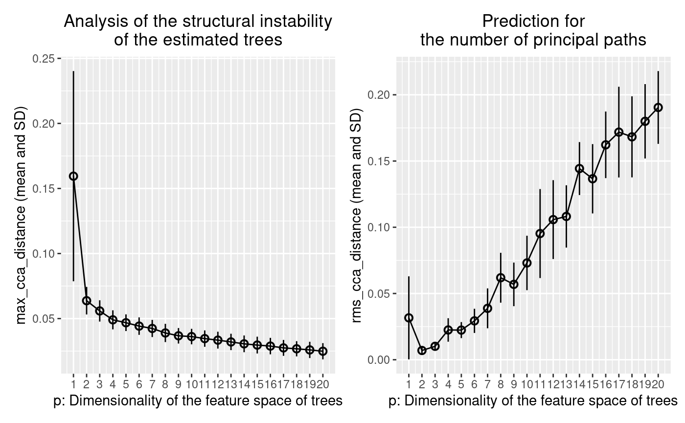
Figure 3. The output for the tree-like data shown in Figure 1
2.2. Less tree-like, noisy toy data
We can analyze the second toy data in the same manner.
fit.less_tree_like <- treefit::treefit(list(expression=star.less_tree_like),
                                       name="less-tree-like")
# Save the analytsis result to use other tutorials.
saveRDS(fit.less_tree_like, "fit.less_tree_like.rds")
fit.less_tree_like
## $name
## [1] "less-tree-like"
##
## $max_cca_distance
## p mean standard_deviation
## 1 1 0.47343135 0.19730822
## 2 2 0.25114667 0.05233404
## 3 3 0.21527536 0.03786608
## 4 4 0.19175361 0.03588504
## 5 5 0.17465724 0.03744595
## 6 6 0.15146467 0.03420347
## 7 7 0.12901100 0.03597212
## 8 8 0.12249087 0.03289082
## 9 9 0.11790721 0.03092478
## 10 10 0.10796651 0.02653031
## 11 11 0.10093718 0.02469578
## 12 12 0.09684883 0.02332913
## 13 13 0.09208538 0.02384131
## 14 14 0.08816012 0.02104161
## 15 15 0.08590189 0.02007525
## 16 16 0.08300275 0.01985852
## 17 17 0.08190812 0.02001626
## 18 18 0.08028083 0.01939304
## 19 19 0.07830362 0.01811760
## 20 20 0.07478951 0.01679053
##
## $rms_cca_distance
## p mean standard_deviation
## 1 1 0.2611212 0.23153838
## 2 2 0.1020510 0.03613444
## 3 3 0.2085653 0.10518241
## 4 4 0.2625540 0.08417689
## 5 5 0.2826318 0.09317319
## 6 6 0.3071232 0.07315173
## 7 7 0.3161327 0.06276053
## 8 8 0.3035636 0.05866871
## 9 9 0.3141727 0.04856548
## 10 10 0.3164844 0.04285037
## 11 11 0.3288808 0.04072976
## 12 12 0.2995099 0.04169197
## 13 13 0.3087054 0.04200793
## 14 14 0.3119395 0.03907616
## 15 15 0.3206773 0.03821475
## 16 16 0.3282625 0.03741899
## 17 17 0.3393654 0.03370764
## 18 18 0.3479858 0.03610781
## 19 19 0.3464760 0.03478315
## 20 20 0.3473163 0.03663275
##
## $n_principal_paths_candidates
## [1] 3 9 13 20
##
## attr(,"class")
## [1] "treefit"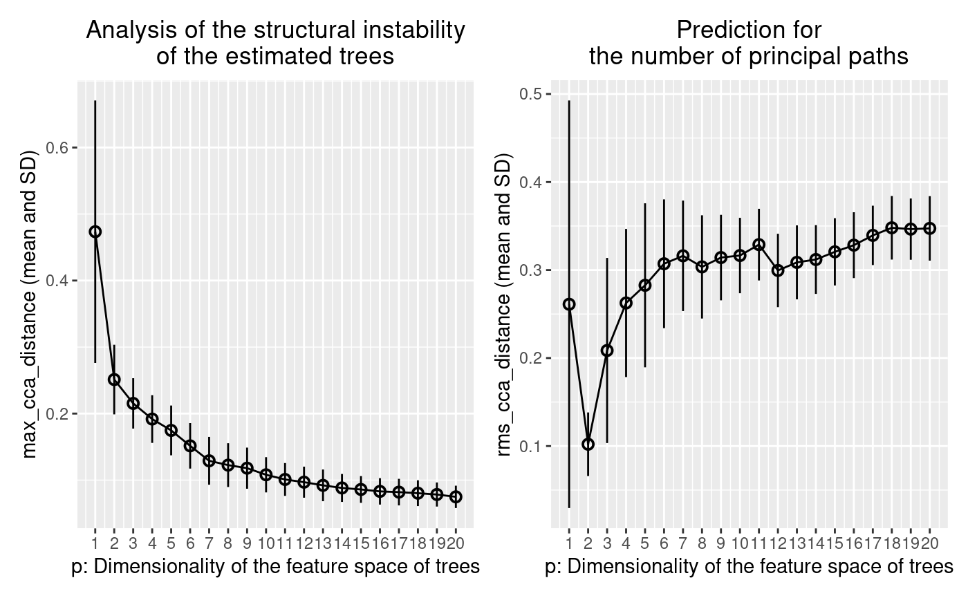
Figure 4. The output for the noisy data shown in Figure 2
2.3. Comparing two results
We can compare different results by passing all results to plot() as follows:
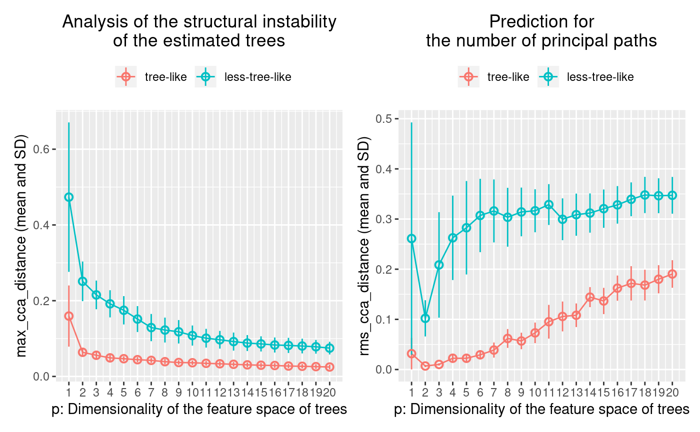
Figure 5. Comparison of the plots shown in Figure 3 and Figure 4.
3. Interpreting the results
Before interpreting the previous results, we briefly summarize the process of the Treefit analysis that consists of the following three steps.
First, Treefit repeatedly “perturbs” the input data (i.e., adds some small noise to the original row count data or normalized expression data) in order to produce many slightly different datasets that may have been acquired in the biological experiment.
Second, for each dataset, Treefit calculates a distance matrix that represents the dissimilarities between sample cells and then constructs a tree from each distance matrix. The current version of Treefit computes a minimum spanning tree (MST) that has been widely used for trajectory inference.
Finally, Treefit evaluates the goodness-of-fit between the data and tree models. The underlying idea of this method is that the structure of trees inferred from tree-like data tends to have high robustness to noise, compared to non-tree-like data. Therefore, Treefit measures the mutual similarity between estimated trees in order to check the stability of the tree structures. To this end, Treefit constructs a p-dimensional subspace that extracts the main features of each tree structure and then measuring mutual similarities between the subspaces by using a special type of metrics called the Grassmann distance. In principle, when the estimated trees are mutually similar in their structure, the mean and standard deviation (SD) of the Grassmann distance are small.
Although the word “Grassmann distance” may sound so unfamiliar to some readers, the concept appears in different disguises in various practical contexts. For example, the Grassmann distance has a close connection to canonical correlation analysis (CCA). Treefit provides two Grassmann distances $max_cca_distance and $rms_cca_distance that can be used for different purposes as we now explain.
3.1. Estimating the tree-likeness of data
The Treefit analysis using the first Grassmann distance $max_cca_distance (shown in the left panel of Figure 5) tells us the goodness-of-fit between data and tree models. In principle, as mentioned earlier, if the mean and SD of $max_cca_distance are small, then this means that the estimated trees are mutually similar in their structure. As can be observed, the distance changes according to the dimensionality p of the feature space, but $max_cca_distance has the property that the value decreases monotonically as p increases for any datasets.
Comparing the Treefit results for the two datasets, we see that the mean Grassmann distance for the first data does not fall below the second one regardless of the value of p and that the SD of the Grassmann distance for the first data is very small compared to the second data. These results imply that the estimated tree structures are very robust to noise in the first case but not in the second case. Thus, Treefit has verified that the first data are highly tree-like while the second data are not.
3.2. Predicting the number of principal paths in the underlying tree
The Treefit analysis using the other Grassmann distance $rms_cca_distance (shown in the right panel of Figure 5) is useful to infer the number of “principal paths” in the best-fit tree. From a biological perspective, this analysis can be used to discover a novel or unexpected cell type from single-cell gene expression (for details, see vignette("working-with-seurat")).
Unlike the previous Grassmann distance, the mean value of $rms_cca_distance can fluctuate depending on the value of p. Interestingly, we can predict the number of principal paths in the best-fit tree by exploring for which p the distance value reaches “the bottom of a valley” (i.e., attains a local minimum). More precisely, when $rms_cca_distance attains a local minimum at a certain p, the value p+1 indicates the number of principal paths in the best-fit tree. $n_principal_paths_candidates has these p+1 values. We don’t need to calculate them manually. When Treefit produces a plot having more than one valleys, the smallest p is usually most informative for the prediction. The smallest p+1 value can be obtained by $n_principal_paths_candidates[1].
Comparing the Treefit results for the two datasets, we first see that both plots attains a local minimum at p=2. This means that for both datasets the best-fit tree has p+1=3 principle paths, which is correct because both were generated from the same star tree with three arms. Another important point to be made is that the SD of the Grassmann distance for the first data is very small at p=2 compared to that for the second data; in other words, Treefit made this prediction more confidently for the first dataset than for the second one. This result is reasonable because the first dataset is much less noisy than the second one. Thus, Treefit has correctly determined the number of principal paths in the underlying tree together with the goodness-of-fit for each dataset.